Evaluating Motion Consistency by Fréchet Video Motion Distance (FVMD)

In this blog post, we introduce a promising new metric for video generative models, Fréchet Video Motion Distance (FVMD), which focuses on the motion consistency of generated videos.

Introduction

Recently, diffusion models have demonstrated remarkable capabilities in high-quality image generation. This advancement has been extended to the video domain, giving rise to text-to-video diffusion models, such as Pika, Runway Gen-2, and Sora .

Despite the rapid development of video generation models, research on evaluation metrics for video generation remains insufficient (see more discussion on our blog). For example, FID-VID and FVD are commonly used video metrics. FID-VID focuses on visual quality by comparing synthesized frames to real ones, ignoring motion quality. FVD adds temporal coherence by using features from a pre-trained action recognition model, Inflated 3D Convnet (I3D) . Recently, VBench introduces a 16-dimensional evaluation suite for text-to-video generative models. However, VBench’s protocols for temporal consistency, like temporal flickering and motion smoothness, favor videos with smooth or static movement, neglecting high-quality videos with intense motion, such as dancing and sports videos.

Simply put, there is a lack of metrics specifically designed to evaluate the complex motion patterns in generated videos. The Fréchet Video Motion Distance (FVMD) addresses this gap.

The code is available at GitHub.

Fréchet Video Motion Distance (FVMD)

The overall pipeline of the Fréchet Video Motion Distance (FVMD) that measures the discrepancy in motion features between generated videos and ground-truth videos.

The core idea of FVMD is to measure temporal motion consistency based on the patterns of velocity and acceleration in video movements. First, motion trajectories of key points are extracted using the pre-trained model PIPs++ , and their velocity and acceleration are computed across frames. Motion features are then derived from the statistics of these vectors. Finally, the similarity between the motion features of generated and ground truth videos is measured using the Fréchet distance .

Video Key Points Tracking

Key point tracking results on the TikTok datasets using PIPs++ .

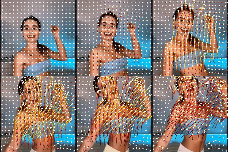
To construct video motion features, key point trajectories are first tracked across the video sequence using PIPs++. For a set of $m$ generated videos, denoted as $\lbrace X^{(i)} \rbrace_{i=1}^m$, the tracking process begins by truncating longer videos into segments of $F$ frames with an overlap stride of $s$. For simplicity, segments from different videos are put together to form a single dataset $\lbrace x_{i} \rbrace_{i=1}^n$. Then, $N$ evenly-distributed target points in a grid shape are queried on the initial frames For example, $F=16, s=1, N=400$ are used as default parameters to extract consecutive short segments. and their trajectories are estimated across the video segments, resulting in a tensor $\hat{Y} \in \mathbb{R}^{F \times N \times 2}$.

Key Points Velocity and Acceleration Fields

FVMD proposes using the velocity and acceleration fields across frames to represent video motion patterns. The velocity field $\hat{V} \in \mathbb{R}^{F \times N \times 2}$ measures the first-order difference in key point positions between consecutive frames with zero-padding:

\[\hat{V} = \texttt{concat}(\boldsymbol{0}_{N\times 2}, \hat{Y}_{2:F} - \hat{Y}_{1:F-1}) \in \mathbb{R}^{F \times N \times 2},\]

The acceleration field $\hat{A} \in \mathbb{R}^{F \times N \times 2}$ is calculated by taking the first-order difference between the velocity fields in two consecutive frames, also with zero-padding:

\[\hat{A} = \texttt{concat}(\boldsymbol{0}_{N\times 2}, \hat{V}_{2:F} - \hat{V}_{1:F-1}) \in \mathbb{R}^{F \times N \times 2}.\]

Motion Feature

To obtain compact motion features, the velocity and acceleration fields are further processed into spatial and temporal statistical histograms.

First, the magnitude and angle for each tracking point in the velocity and acceleration vector fields are computed respectively. Let $\rho(U)$ and $\phi(U)$ denote the magnitude and angle of a vector field $U$, where $U \in \mathbb{R}^{F \times N \times 2}$ and $U$ can be either $\hat{V}$ or $\hat{A}$.

\[\begin{aligned} \rho(U)_{i, j} &= \sqrt{U_{i,j,1}^2 + U_{i,j,2}^2}, &\forall i \in [F], j \in [N], \\ \phi(U)_{i, j} &= \left| \tanh^{-1}\left(\frac{U_{i, j,1}}{U_{i, j,2}}\right) \right|, &\forall i \in [F], j \in [N]. \end{aligned}\]

Then, FVMD quantizes magnitudes and angles into discrete bins (8 for angles and 9 for magnitudes), which are then used to construct statistical histograms and extract motion features. It adopts dense 1D histograms The 1D histogram approach is inspired by the HOG (Histogram of Oriented Gradients) approach , which counts occurrences of gradient orientation in localized portions of an image. by aggregating magnitude values into 1D histograms corresponding to the quantized angles. Specifically, the $F$-frame video segments are divided into smaller volumes of size $f \times k \times k$, where $f$ is the number of frames and $k$ the number of tracking points. Within each small volume, every tracking point’s magnitude is summed into its corresponding angle bin, resulting in an 8-point histogram per volume. Eventually, the histograms from all volumes are combined to form the final motion feature The shape of the dense 1D histogram is $ \lfloor \frac{F}{f} \rfloor \times \lfloor \frac{\sqrt{N}}{k} \rfloor \times \lfloor \frac{\sqrt{N}}{k} \rfloor \times 8$..

Dense 1D histograms are used for both velocity and acceleration fields, and the resulting features are concatenated to form a combined motion feature for computing similarity.

click here for 2D histogram construction

FVMD also explores quantized 2D histograms but opts to use the dense 1D histograms for the default configuration due to their superior performance. In this approach, the corresponding vector fields of each volume are aggregated to form a 2D histogram, where $x$ and $y$ coordinates represent magnitudes and angles, respectively. The 2D histograms from all volumes are then concatenated and flattened into a vector to serve as the motion feature. The shape of the quantized 2D histogram is $ \lfloor \frac{F}{f} \rfloor \times \lfloor \frac{\sqrt{N}}{k} \rfloor \times \lfloor \frac{\sqrt{N}}{k} \rfloor \times 72$, where the number 72 is derived from 8 discrete bins for angle and 9 bins for magnitude.

Visualizations

If two videos are of very different quality, their histograms should look very different to serve as a discriminative motion feature. Let’s take a look at what they look like for the videos in real life.

Raw videos and tracking results on the TikTok datasets . Left: Ground-truth video. Middle and right: Generated videos for the same scene of worse (middle) and better (right) quality, respectively.

Above, we show three pieces of video from the TikTok dataset with very different visual qualities for the same scene. One can easily spot their differences in motion patterns. Next, we show the 1D histograms based on the velocity field of the videos.

Dense 1D histograms for the velocity fields of the videos. Left: Ground-truth video. Middle and right: Generated videos for the same scene of worse (middle) and better (right) quality, respectively.

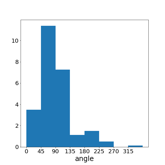
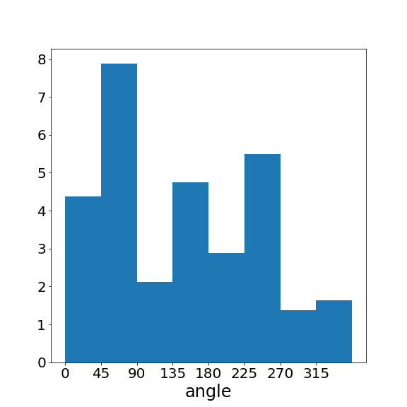
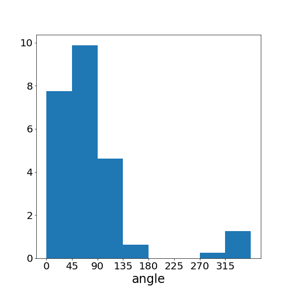
The low-quality video has more abrupt motion changes, resulting in a substantially greater number of large-angle velocity vectors. Therefore, the higher-quality video (right) has a motion pattern closer to the ground-truth video (left) than the lower-quality video (middle). This is exactly what we want to observe in the motion features! These features can capture the motion patterns effectively and distinguish between videos of different qualities.

click here for 2D histogram result

Dense 2D histograms for the velocity fields of the videos. Left: ground-truth video. Middle and right: Generated videos of worse and better quality, respectively.

We can observe similar patterns in the 2D histograms. The higher-quality video (right) has a motion pattern closer to the ground-truth video (left) than the lower-quality video (middle). The unnatural jittering and unsmooth motion in the lower-quality video lead to more frequent large-magnitude velocity vectors, as captured by the 2D histograms.

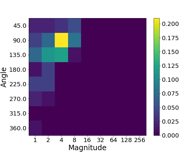
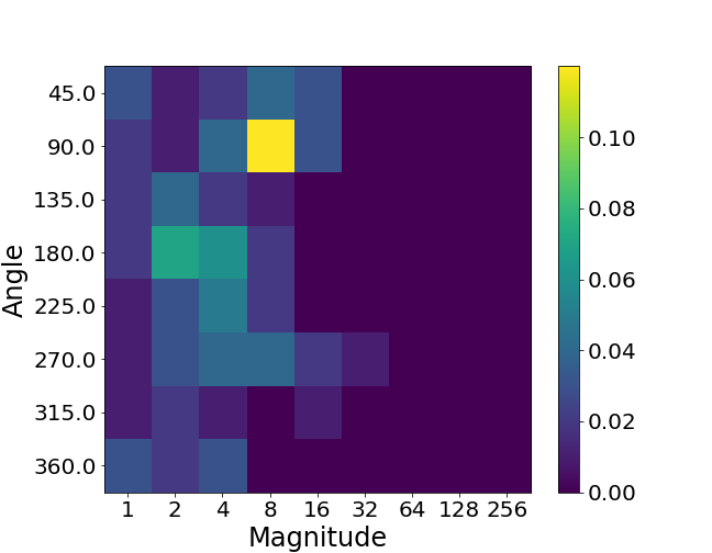
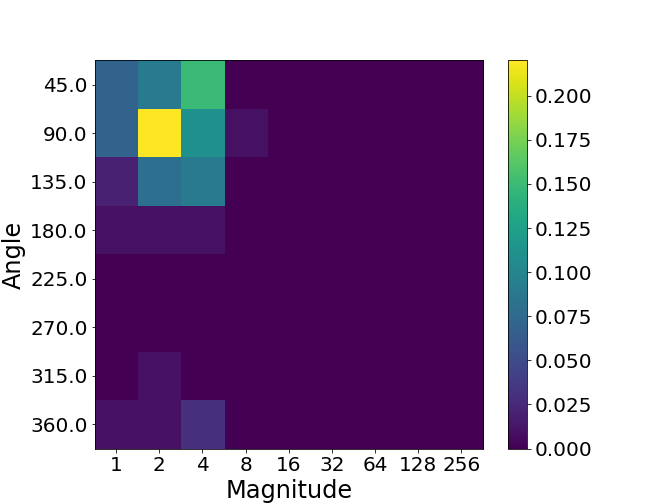
Fréchet Video Motion Distance

After extracting motion features from video segments of generated and ground-truth video sets, FVMD measures their similarity using the Fréchet distance , which explains the name Fréchet Video Motion Distance (FVMD). To make the computation tractable, multi-dimensional Gaussian distributions are used to represent the motion features, following previous works . Let $\mu_{\text{gen}}$ and $\mu_{\text{data}}$ be the mean vectors, and $\Sigma_{\text{gen}}$ and $\Sigma_{\text{data}}$ be the covariance matrices of the generated and ground-truth videos, respectively. The FVMD is defined as:

\[d_F = ||\mu_{\text{data}}-\mu_{\text{gen}}{||}_2^2 + \mathrm{tr}\left(\Sigma_{\text{data}} + \Sigma_{\text{gen}} -2(\Sigma_{\text{data}}\Sigma_{\text{gen}})^{\frac{1}{2}}\right)\]

Experiments

The ultimate aim of a video evaluation metric is to align with human perception. To validate the effectiveness of FVMD, a series of experiments is conducted in the paper, including sanity check, sensitivity analysis, and quantitative comparison with existing metrics. Large-scale human studies are also performed to compare the performance of FVMD with other metrics.

Sanity Check

To verify the efficacy of the extracted motion features in representing motion patterns, a sanity check is performed in the FVMD paper. Motion features based on velocity, acceleration, and their combination are used to compare videos from the same dataset and different datasets.

As sample size increases, same-dataset discrepancies (BAIR vs BAIR) converge to zero, while cross-dataset discrepancies (TIKTOK vs BAIR) remain large, verifying the soundness of the FVMD metric.

When measuring the FVMD of two subsets from the same dataset, it converges to zero as the sample size increases, confirming that the motion distribution within the same dataset is consistent. Conversely, the FVMD remains higher for subsets from different datasets, showing that their motion patterns exhibit a larger gap compared to those within the same dataset.

Sensitivity Analysis

Moreover, a sensitivity analysis is conducted to evaluate if the proposed metric can effectively detect temporal inconsistencies in generated videos, i.e., being numerically sensitive to temporal noises. To this end, artificially-made temporal noises are injected to the TikTok dancing dataset and FVMD scores are computed to assess its sensitivity to data corruption.

The FVMD scores in the presence of various temporal noises are presented.

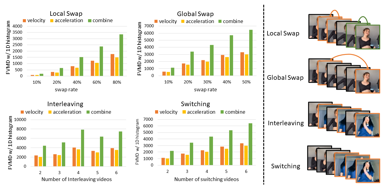
Across the four types of temporal noises injected into the dataset There are four types of temporary noises in the FVMD paper: 1) local swap: swapping a fraction of consecutive frames in the video sequence, 2) global swap: swapping a fraction of frames in the video sequence with randomly chosen frames, 3) interleaving: weaving the sequence of frames corresponding to multiple different videos to obtain new videos, 4) switching: jumping from one video to another video. , FVMD based on combined velocity and acceleration features demonstrates the most reliable performance. It shows a strong negative correlation with noise level, indicating FVMD’s sensitivity to temporal noise and its effectiveness in detecting temporal inconsistencies in generated videos.

Quantitative Results

Further, FVMD provides a quantitative comparison of various video evaluation metrics on TikTok dataset . Fifty videos are generated using different checkpoints named (a) through (e) The video samples are reproduced from the following models: (a) is from Magic Animate ; (b), (c), and (e) are from Animate Anyone , each with different training hyperparameters; and (d) is from DisCo . and their performance is measured using the FVD , FID-VID , VBench , and FVMD metrics. Note that the models (a) to (e) are sorted based on human ratings collected through a user study, from worse to better visual quality (model (e) has the best visual quality and model (a) has the worst). This allows for a comparison of how well the evaluation metrics align with human judgments.

Video samples created by various video generative models trained on the TikTok dataset are shown to compare the fidelity of different evaluation metrics.

Metrics	Model (a)	Model (b)	Model (c)	Model (d)	Model (e)	Human Corr.↑
FID↓	73.20 (3rd)	79.35 (4th)	63.15 (2nd)	89.57 (5th)	18.94 (1st)	0.3
FVD↓	405.26 (4th)	468.50 (5th)	247.37 (2nd)	358.17 (3rd)	147.90 (1st)	0.8
VBench↑	0.7430 (5th)	0.7556 (4th)	0.7841 (2nd)	0.7711 (3rd)	0.8244 (1st)	0.9
FVMD↓	7765.91 (5th)	3178.80 (4th)	2376.00 (3rd)	1677.84 (2nd)	926.55 (1st)	1.0

FVMD ranks the models correctly in line with human ratings and has the highest correlation to human perceptions. Moreover, FVMD provides distinct scores for video samples of different quality, showing a clearer separation between models.

Human Study

In the paper, large-scale human studies are conducted to validate that the proposed FVMD metric aligns with human perceptions. Three different human pose-guided generative models are fine-tuned: DisCo , Animate Anyone , and Magic Animate . These models, with distinct architectures and hyper-parameter settings, yield over 300 checkpoints with varying sample qualities. Users are then asked to compare samples from each pair of models to form a ground-truth user score. All checkpoints are also automatically evaluated using the FVMD metric, and the results are compared with FID-VID , FVD , SSIM , PSNR , and VBench . The correlation between the scores given by each metric and the ground-truth user scores is calculated to further assess the performance of each metric.

Following the model selection strategy in , two settings for the human studies are designed. The first setup is One Metric Equal. In this approach, a group of models with nearly identical scores based on a selected metric is identified. Namely, the selected models’ generated samples are considered to have similar visual quality compared to the reference data, according to the selected metric. This setup investigates whether the other metrics and human raters can effectively differentiate between these models.

The second setting, One Metric Diverse, evaluates the agreement among different metrics when a single metric provides a clear ranking of the performances of the considered video generative models. Specifically, model checkpoints whose samples can be clearly differentiated according to the given metric are selected to test the consistency between this metric, other metrics, and human raters.

Table 1: Pearson correlation for the One Metric Equal experiments.

Table 2: Pearson correlation for One Metric Diverse experiments.

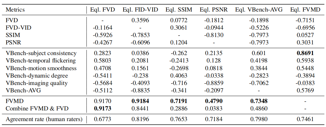
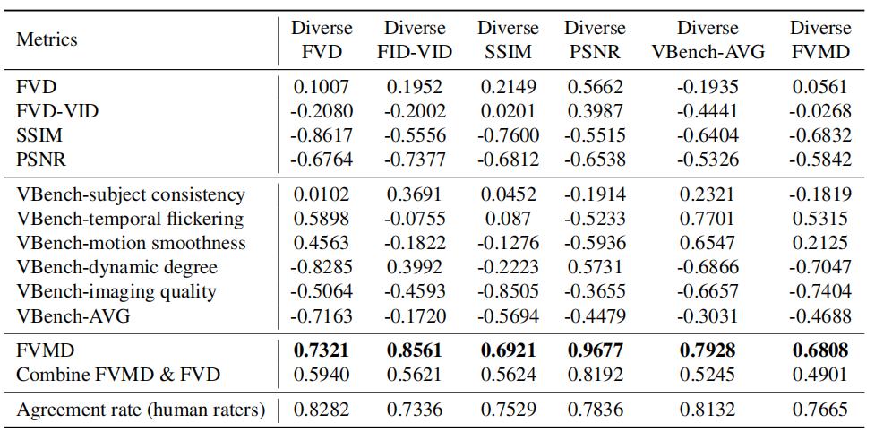
The Pearson correlations range in [-1, 1], with values closer to -1 or 1 indicating stronger negative or positive correlation, respectively. The agreement rate among raters is reported as a percentage from 0 to 1. A higher agreement rate indicates a stronger consensus among human raters and higher confidence in the ground-truth user scores. The correlation is higher-the-better for all metrics in both One Metric Equal and One Metric Diverse settings. Overall, FVMD demonstrates the strongest capability to distinguish videos when other metrics fall short.

Summary

In this blog, we give a brief summary of the recently-proposed Fréchet Video Motion Distance (FVMD) metric and its advantages over existing metrics. FVMD is designed to evaluate the motion consistency of generated videos by comparing the discrepancies of velocity and acceleration patterns between generated and ground-truth videos. The metric is validated through a series of experiments, including a sanity check, sensitivity analysis, quantitative comparison, and large-scale human studies. The results show that FVMD outperforms existing metrics in many aspects, such as better alignment with human judgment and a stronger capability to distinguish videos of different quality.